Conversion technologies¶

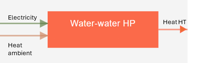
Conversion technologies are systems that transform one or more energy carriers into different types — for example, a gas boiler converting natural gas to heat. Each technology is defined by:

• Technical parameters: efficiencies and technical limits.
• Financial and environmental parameters: investment costs (CAPEX), operational costs (OPEX), and embodied emissions.

For parameters, see Conversion technology parameters.

Technology modes¶

A mode represents a specific operational regime with its own set of inputs, outputs, and efficiencies. A single technology can have multiple modes to reflect different seasonal or functional behaviors.

• Example: a reversible heat pump has a heating mode and a cooling mode, each with a distinct coefficient of performance (COP).
• Configuration: technical parameters are applied at the mode level, to allow for this granular operational modeling.

Primary vs. non-primary modes¶

To ensure costs accurately reflect physical hardware requirements, modes are categorized:

• Primary mode: a mode whose sizing must be reflected in cost and CO2 emissions. The technology's costs are derived from the capacity requirements of these modes.
• Non-primary mode: a "bonus" mode. Its capacity does not increase the technology's investment or operational costs, or its CO2 emissions — it represents secondary use of existing hardware.

Mode capacity¶

The capacity of a specific mode is the maximum hourly sum of all primary outputs recorded for that mode.

You can choose between two sizing behaviors:

• Optimize mode capacity: optionally enter a minimum and/or maximum installed capacity; the optimal capacity is selected within this range. If a minimum capacity is specified and the default option is selected, the installed capacity can be 0 or greater than the minimum.
• Specify mode capacity: installed capacity is held at a fixed value. Operating capacity (which does not influence investment costs) may be equal to or lower than installed capacity.

Technology capacity¶

The technology capacity represents the installed capacity of the unit and is used for cost and CO2 calculations. It equals the maximum total primary output summed across all primary modes at any single point in time.

Example calculation¶

• Mode A peak (primary): 100 kW at hour 5.
• Mode B peak (primary): peak of 200 kW at hour 10.
• Peak of the sum of primary modes: at hour 8, modes A and B produce a combined 250 kW.

Result: the technology capacity is 250 kW.

Mode efficiency¶

The efficiency of a mode indicates energy dissipation within systems. The sum of output efficiencies represents the mode's total efficiency:

• A total efficiency of 100% means useful energy is conserved within the system.
• A total efficiency below 100% indicates useful energy is lost in the system — for example, heat losses in the technology, which are not modeled as a "waste heat" flow.
• A total efficiency above 100% indicates useful energy is created within the system — for example, useful heat extracted from the environment, which is not modeled as an "ambient air" flow.

Example: heat pump¶

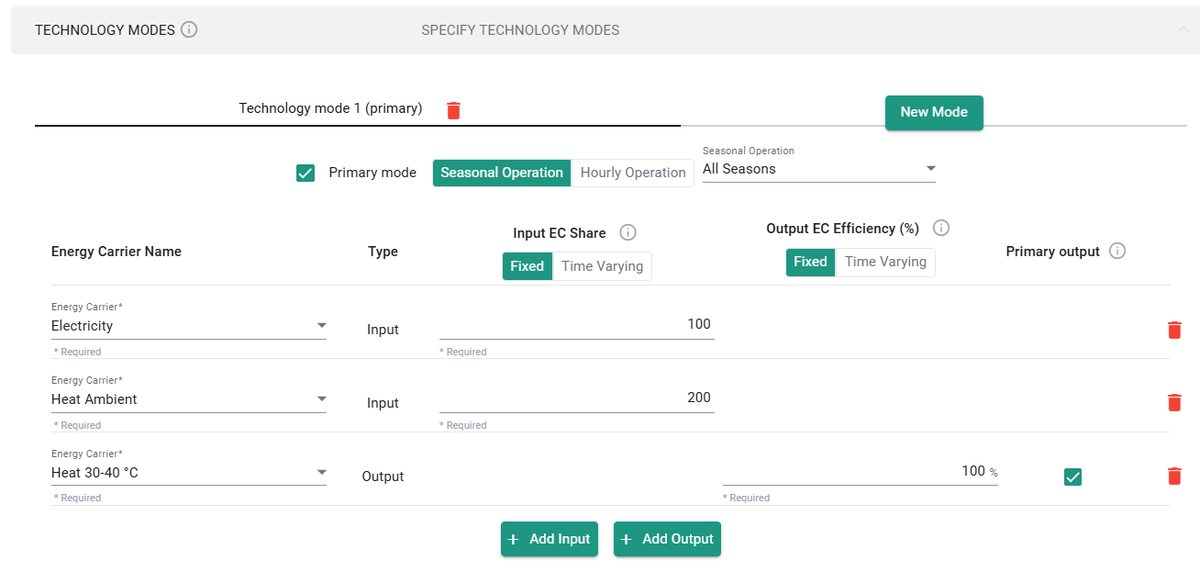
The efficiency of a standard input (with two inputs) is set as follows:

The calculation is:

Output EC(i) = Sum of inputs × efficiency output(i)

HT heat = (100 + 200) × 100% = 300

In this case, 100 units of electricity and 200 units of ambient heat produce 300 units of HT heat. This corresponds to a yearly COP of 3.

In the app, the numbers are entered as follows:

Example: chiller¶

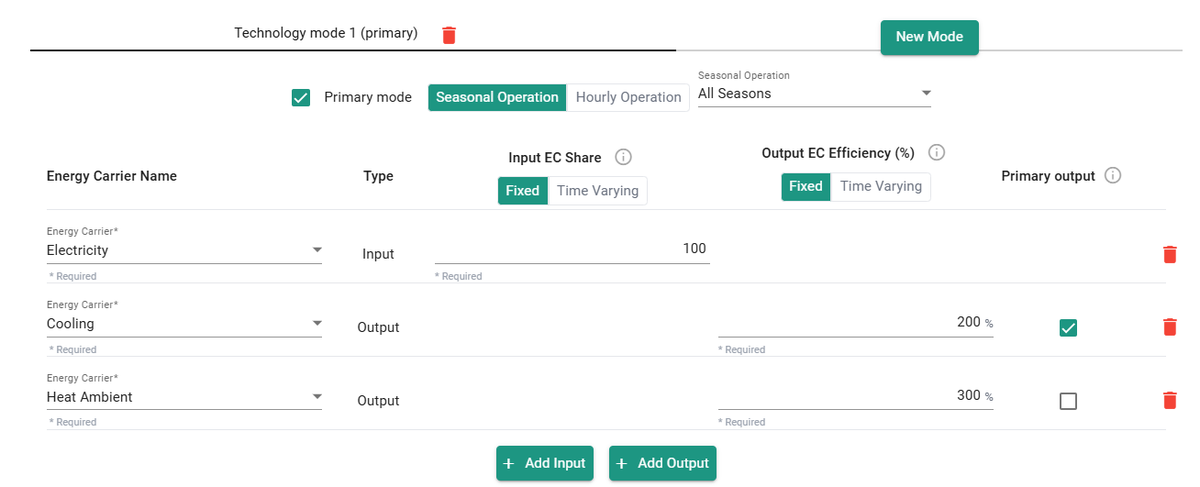
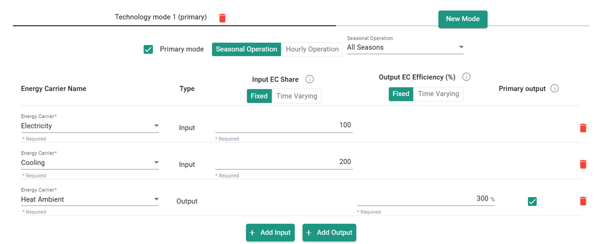
For chillers, there are two ways to model cooling energy. The first method treats cooling energy as a service, meaning the energy is generated and supplied. For example, when modeling a chiller with an energy efficiency ratio (EER) of 2, the process is as follows:

This means that an input of 100 units of electricity produces 200 units of cooling (based on an EER of 2) and 300 units of heating (assuming the electricity is fully dissipated as heat).

100 units of electricity give, in this case, 300 units of HT heat and 200 units of cooling, from which an EER of 2 is calculated. Here, the cumulative output efficiency is greater than 100%, which reflects the "creation" of energy — because cooling energy is treated as an additional service.

In the app, the numbers are entered as follows:

Alternative method: chiller¶

There's also an alternative method where cooling energy is treated as an extraction of energy demand. To use this method, set the cooling demand to "reversed." In this case, the chiller can be modeled as a heat pump with an EER of 2 (or a COP of 3).

In the app, the numbers are entered as follows:

For this method, it's crucial that the reverse box is ticked for the cooling demand in the Energy Demands step — this treats cooling as an extraction of heat.

Simultaneity of operation¶

Different modes can operate simultaneously. To prevent this, leave the simultaneous checkbox unchecked, indicating the mode cannot run with others. This may increase optimization time.

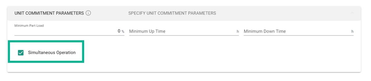
Alternatively, a less computationally intensive option is to define a different seasonal or hourly operation for each mode.

Some advanced parameters are not available to all plan tiers, but can be added through add-on options. Contact customer support for a demo and to discuss customizing these options to your needs.

Seasonal and hourly parameters¶

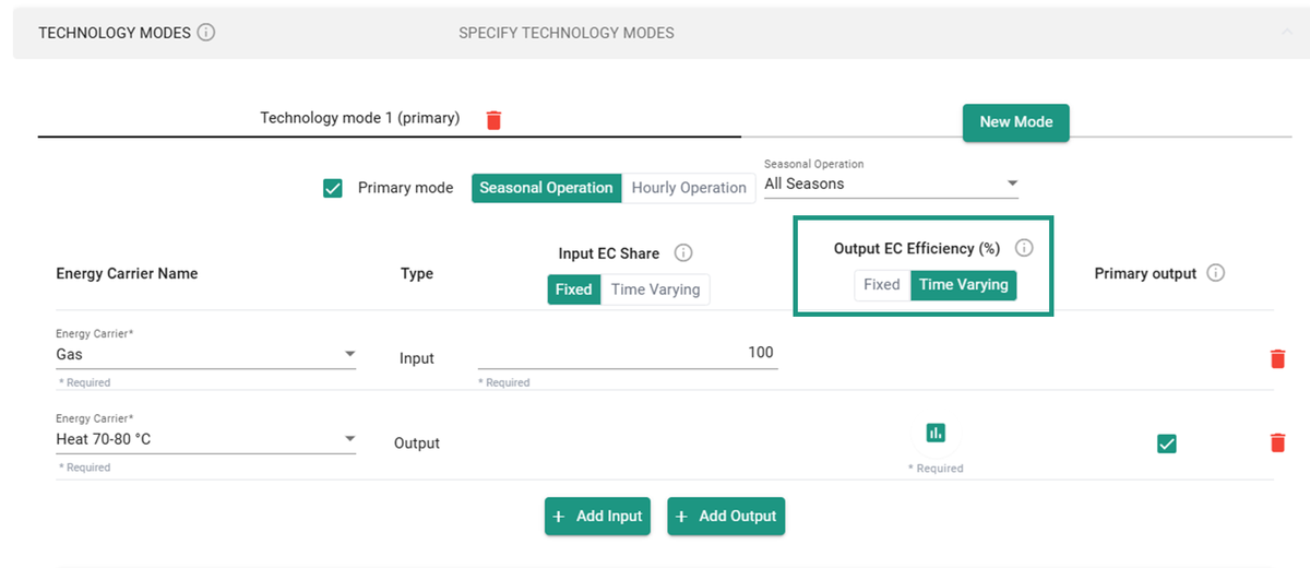
You can enter time-varying efficiencies, either as monthly or hourly values. To do so, select Time varying instead of Fixed for the output EC efficiency.

The case of heat pumps¶

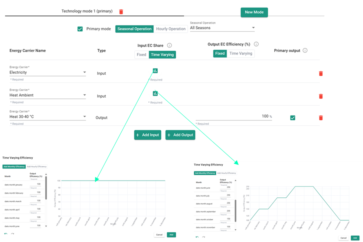
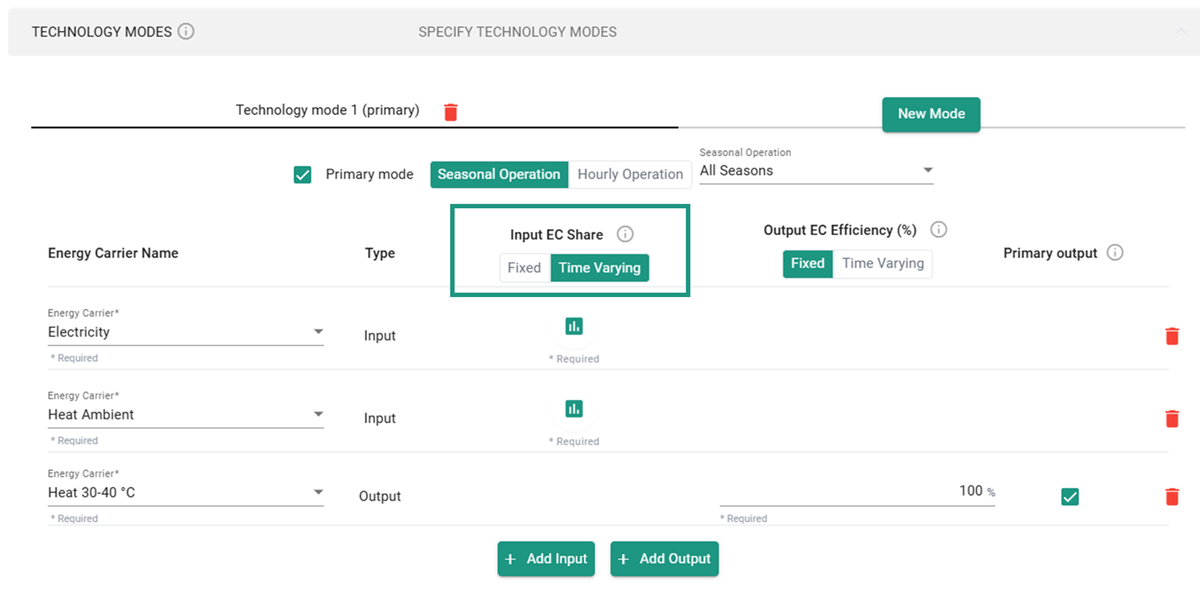
For heat pumps, if you want to apply a time-varying COP, modify the input EC share rather than the output efficiency — the input EC share is what defines the COP (= heat HT / electricity). See the example below: